The Question

Act I

Does gaining legal access to alcohol make young people more likely to die?

In the United States, the minimum legal drinking age (MLDA) is 21.

Should it be lower? If legal access raises deaths, a birthday rule is a life-and-death policy lever.

Open with the policy question. Ask the room: would lowering the MLDA cost lives? Bright lines are everywhere: voting at 18, Medicare eligibility at 65, legal drinking at 21. This chapter shows how to turn such lines into evidence.

Rigid rules look like the enemy of experiments — yet they create one

• A bureaucratic cutoff seems to leave nothing to chance
• But someone aged 20 years and 11 months is a near twin of someone aged 21 and 1 month
• Only one of them may legally buy a drink

Near the line, the rule — not the person — decides who is treated.

Finish-line analogy: a sprinter at 9.99 seconds and one at 10.01 seconds are equally talented, but only one gets the medal. The medal is the treatment, assigned by the line. A cutoff therefore mimics a lottery for the people standing right next to it.

Monthly death rates step up right at the 21st birthday

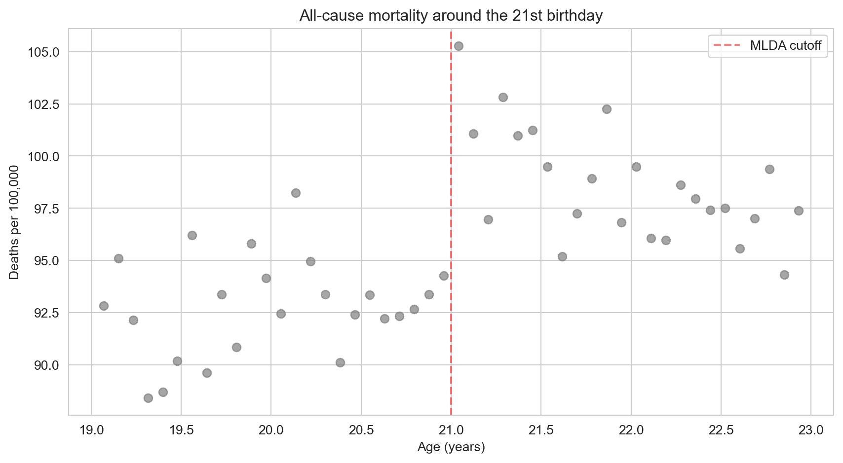
All-cause deaths per 100,000, one dot per monthly age cell; the dashed line marks age 21.

Each dot is one month of age. Below 21 the rates sit in the low-to-mid 90s; the cells just after 21 are among the highest in the sample. Ask: is this a coincidence of age, or the effect of legal access? The rest of the lecture makes that judgement rigorous.

Our route through the chapter

• The question — how a birthday rule can act like a natural experiment
• The investigation — the sharp RD design and regression; the MLDA mortality case study; robustness checks; fuzzy RD and Boston’s exam schools
• The resolution — what RD can and cannot claim, and the traps to avoid

Learning objectives: explain how cutoffs create natural experiments; define running variable, cutoff, and treatment indicator; distinguish sharp and fuzzy RD; estimate effects with polynomial regression at a discontinuity; check robustness with bandwidth and specification choices; interpret RD as a local effect at the cutoff.

Three ingredients define every RD design

Running variable

The continuous score that decides treatment — here, age \(a\).

Cutoff

The value where treatment switches — here, 21.

Treatment indicator

\(D_a = 1\) at or above the cutoff, \(0\) below it.

Name these three and you have described the design.

Other cutoffs: an exam score of 70 for passing, age 65 for Medicare, an income limit for a benefit. In the data, age is agecell (or age, centred at 21) and the treatment dummy is over21.

Four more words we will use all lecture

Term	Plain meaning
Sharp vs. fuzzy RD	Treatment flips fully at the cutoff vs. only its probability jumps
Continuity assumption	Without treatment, outcomes would pass smoothly through the cutoff
Bandwidth	How far from the cutoff we let the data reach
Placebo test	Check an outcome that should not jump — it must stay flat

Sharp/fuzzy says how treatment moves; the other three keep the jump honest.

Analogies: sharp RD is a light switch, fuzzy RD a dimmer. Continuity is a smooth road — a sudden bump means something was placed there. Bandwidth is zooming a photo in or out. A placebo test is checking that a medicine does not change hair colour.

The Investigation

Act II

At the cutoff, drinkers and non-drinkers never share an age

Age	Legal access to alcohol
20 years, 11 months	0%
21 years, 0 months	100%

There is no age at which we can compare treated and untreated people side by side.

RD has no overlap — so it cannot work by matching people with the same age.

In Chapter 2, regression compared treated and untreated people with the same values of the controls. Here that is impossible: everyone over 21 is treated, everyone under 21 is not. The design must lean on something else — the shape of the trend on each side.

RD does not “control for” age — it extrapolates each side to the line

Regression with controls

• Compare treated and untreated at the same value of a control
• Needs both groups at every value

Regression discontinuity

• Fit the trend separately on each side
• Project both trends to 21 and read the gap

Because RD extrapolates, the shape of the fitted trend matters.

This is the chapter’s main misconception. A straight line projected to 21 and a curved line projected to 21 can land at different heights — which is why we will vary the functional form later.

A birthday flips legal access from 0 to 1

\[D_a = \begin{cases} 1 & \text{if } a \geq 21 \\ 0 & \text{if } a < 21 \end{cases}\]

\(a\) is age (the running variable, agecell); \(D_a\) is the treatment switch (over21).

Treatment is a deterministic function of age: no exceptions, no choice — a sharp RD.

Sharp means the probability of treatment goes from 0% to 100% at the cutoff. Nobody can pick their birthday, which also rules out people sorting themselves to one side of the line.

Age shapes death rates smoothly; only legal access can jump at 21

Age has a smooth path to mortality; the legal-access path is the only one that can create a break.

Age affects mortality directly (maturity, driving experience, lifestyle) — but gradually, month by month. Legal access changes abruptly at 21. If we model the smooth part, what remains at 21 is the causal effect.

Continuity: without the policy, mortality would glide through 21

• Every other influence on death rates changes smoothly with age
• So the outcome trend, absent treatment, has no break at 21
• Any break we see must come from the treatment

A speed bump on a smooth road means someone put it there.

The continuity assumption is the identifying assumption of RD. It fails if something else also switches at 21 — a different law, an insurance rule, a change in how deaths are recorded. Placebo outcomes, later, are how we probe it.

Plot first: a scatter with a line at 21 shows the jump before any model

import pandas as pd                       # pandas → load tables
import matplotlib.pyplot as plt           # matplotlib → draw the scatter

# every course dataset lives in the repo's data/ folder on GitHub
GITHUB_DATA_URL = "https://raw.githubusercontent.com/cmg777/intro2causal/main/data/"
mlda = pd.read_csv(GITHUB_DATA_URL + "ch4/mlda_clean.csv")   # monthly age cells

fig, ax = plt.subplots(figsize=(8, 4.5))                      # one blank panel
ax.scatter(mlda["agecell"], mlda["all"], color="gray")        # death rate vs. age
ax.axvline(21, color="red", linestyle="--")                   # mark the cutoff
plt.show()                                                    # the step at 21 appears

↗ Try it in Colab

Visual inspection is the most important step in RD. If you cannot see a jump in the raw scatter, be suspicious of any regression that claims one. agecell is age in years; all is deaths per 100,000 from all causes. Add ax.set_xlabel("Age (years)") and ax.set_ylabel("Deaths per 100,000") for labels.

One regression measures the jump while holding the age trend fixed

\[M_a = \alpha + \rho \, D_a + \gamma \, a + e_a\]

• \(\rho\) = jump at the cutoff — the causal effect
• \(\gamma\) = the smooth age trend

• \(M_a\) = death rate (all); \(D_a\) = over21
• \(a\) = age centred at 21 (age)

The dummy captures the break; the age term absorbs the smooth slope.

With age centred at 21 (age = agecell − 21), the intercept α is the predicted death rate just below the cutoff and α + ρ the rate just above. In code: pf.feols(“all ~ over21 + age”, vcov=“hetero”).

The vertical gap between the two fitted lines at 21 is the effect

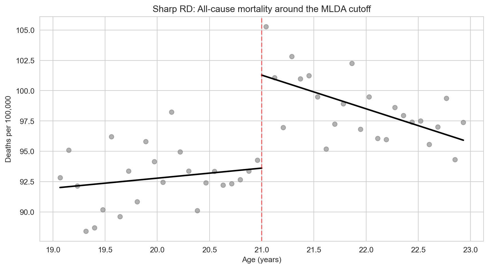
All-cause death rate with a separate straight line fitted on each side of age 21.

Each side gets its own line. Left of 21 the line rises gently; right of 21 it starts much higher and slopes down. If legal access did nothing, the two lines would meet at 21. They do not — the gap is the RD estimate.

The data: 48 monthly age cells around the 21st birthday

Column	Meaning
agecell	Age in years, one cell per month (19 to 23)
age	Age centred at 21 (0 = the cutoff)
over21	Treatment dummy: 1 if 21 or older
all, mva, suicide, internal, alcohol	Deaths per 100,000, by cause
age2, over_age, over_age2	Terms for the quadratic model

Each row is an age, not a person: 24 cells below 21 and 24 above.

US mortality data aggregated into monthly age cells. mva = motor-vehicle accidents; internal = deaths from disease (cancer, heart disease, and so on). The extra polynomial columns are pre-built so the quadratic regression is a one-liner. The CSV has 50 rows, but the two rows at exactly 21 are empty placeholders, so every regression uses 48 cells (pyfixest drops the empty rows).

One pf.feols call estimates the sharp RD

!pip install -q pyfixest                  # pyfixest is not preinstalled in Colab

import pandas as pd                       # pandas → load tables
import pyfixest as pf                     # pyfixest → regressions with robust SEs

GITHUB_DATA_URL = "https://raw.githubusercontent.com/cmg777/intro2causal/main/data/"
mlda = pd.read_csv(GITHUB_DATA_URL + "ch4/mlda_clean.csv")   # MLDA age cells

# death rate on the over-21 switch plus a linear age trend, robust SEs
m = pf.feols("all ~ over21 + age", data=mlda, vcov="hetero")
m.summary()                               # over21 = 7.66 (SE 1.51); Intercept 91.84

↗ Try it in Colab

vcov="hetero" gives heteroskedasticity-robust standard errors. The over21 coefficient is the jump ρ; the intercept is the predicted death rate just below 21; the age slope (−0.97, SE 0.66) is the common trend. t ≈ 5.1 on over21; 48 age cells are used.

Legal access to alcohol raises the death rate at 21

+7.7

extra deaths per 100,000 at the 21st birthday — about 8% above the 91.8 just below

7.66 / 91.84 ≈ 0.083, so an 8% increase in the all-cause death rate, from a single birthday. Robust SE 1.51, t ≈ 5.1 — far beyond noise.

Motor-vehicle accidents carry most of the jump

Cause of death	Jump at 21 (SE)
All causes	7.66 (1.51)
Motor-vehicle accidents	4.53 (0.72)
Suicide	1.79 (0.50)
Alcohol-related (direct)	0.44 (0.21)
Internal causes (disease)	0.39 (0.54)

More than half the extra deaths happen on the road — drunk driving is the main channel.

Linear RD on the full sample, robust SEs, one regression per cause. Across specifications the motor-vehicle jump ranges from about 4.5 to 5.9. Direct alcohol poisoning is small but significant; suicide is modest. Comparing causes is how RD reveals mechanisms.

Diseases ignore the birthday: internal causes do not jump

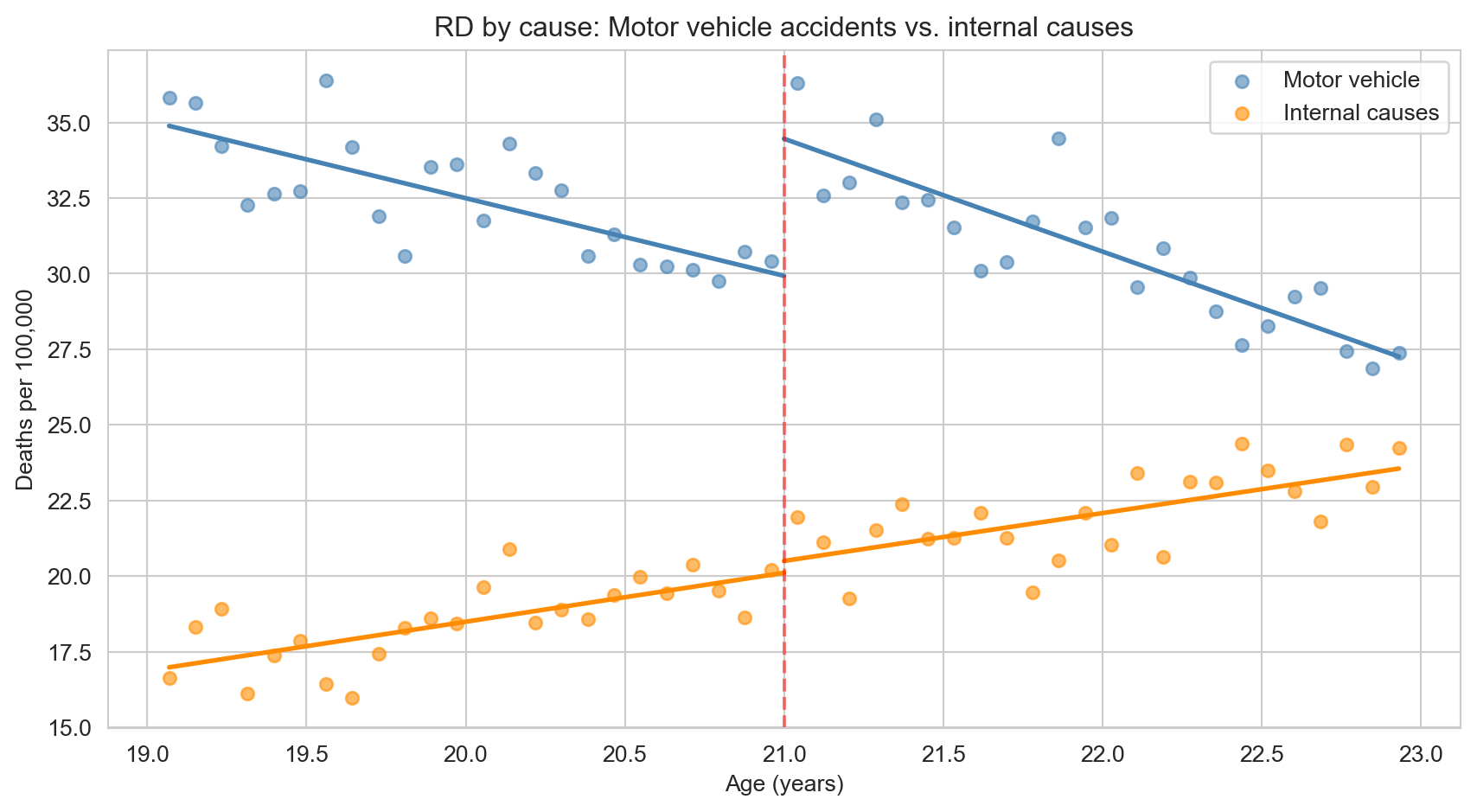
Motor-vehicle deaths (blue) and internal-cause deaths (orange), each with separate lines on either side of 21.

A placebo outcome that stays flat makes the motor-vehicle jump believable.

Cancer and heart disease develop over years; nothing biological happens to them on a 21st birthday. If internal-cause deaths jumped, something else must change at 21 (record-keeping, insurance rules), and we could not trust the motor-vehicle result either. Linear estimate 0.39 (SE 0.54): no jump.

Swapping the outcome turns the same regression into a placebo test

!pip install -q pyfixest                  # pyfixest is not preinstalled in Colab
import pandas as pd                       # pandas → load tables
import pyfixest as pf                     # pyfixest → regressions with robust SEs

GITHUB_DATA_URL = "https://raw.githubusercontent.com/cmg777/intro2causal/main/data/"
mlda = pd.read_csv(GITHUB_DATA_URL + "ch4/mlda_clean.csv")   # MLDA age cells

for y in ["mva", "internal"]:             # a real channel, then a placebo
    m = pf.feols(f"{y} ~ over21 + age", data=mlda, vcov="hetero")   # same RD
    print(y, round(m.coef()["over21"], 2), round(m.se()["over21"], 2))
# mva 4.53 0.72  ·  internal 0.39 0.54

↗ Try it in Colab

The f-string swaps the left-hand variable; everything else is identical. We hope for a large coefficient on mva and a small one on internal. Try suicide, alcohol, or homicide too.

A quadratic lets each side of the cutoff bend in its own way

\[M_a = \alpha + \rho D_a + \gamma_1 a + \gamma_2 a^2 + \delta_1 a D_a + \delta_2 a^2 D_a + e_a\]

Code names: \(a^2\) = age2, \(a D_a\) = over_age, \(a^2 D_a\) = over_age2.

If the jump survives a curved trend, it is not an artefact of forcing a straight line.

A straight ruler may miss a curve; a bendable ruler follows it. The interaction terms (δ) allow the slope and curvature to differ on each side of 21. ρ is still the gap between the two curves at the cutoff, because age is centred there.

Narrowing the window trades precision for comparability

Window around 21	Age cells	Jump (SE)
Full sample (19 to 23)	48	7.66 (1.51)
± 1.5 years	36	8.70 (1.63)
± 1.0 year	24	9.75 (2.06)
± 0.5 years	12	8.88 (3.03)

Closer cells are more alike, but fewer cells mean noisier estimates — the jump stays between 7.7 and 9.8.

Linear RD on all-cause mortality. A narrow bandwidth reduces bias from a mis-specified trend far from the cutoff; a wide one reduces variance. The standard error doubles from 1.51 to 3.03 as the window shrinks to half a year on each side. Reporting several bandwidths is standard practice.

Robustness checks reuse the same call with a new formula or sample

!pip install -q pyfixest                  # pyfixest is not preinstalled in Colab
import pandas as pd                       # pandas → load tables
import pyfixest as pf                     # pyfixest → regressions with robust SEs

GITHUB_DATA_URL = "https://raw.githubusercontent.com/cmg777/intro2causal/main/data/"
mlda = pd.read_csv(GITHUB_DATA_URL + "ch4/mlda_clean.csv")   # MLDA age cells

narrow = mlda[(mlda["agecell"] >= 20) & (mlda["agecell"] <= 22)]   # ages 20–22 only

# interacted quadratic trend on the narrow window, robust SEs
m = pf.feols("all ~ over21 + age + age2 + over_age + over_age2",
             data=narrow, vcov="hetero")
m.summary()                               # over21 = 9.61 (SE 2.29)

↗ Try it in Colab

Two knobs: the formula (linear vs. interacted quadratic) and the data (full vs. narrow window). Change data=narrow to data=mlda for the quadratic on the full sample (9.55, SE 1.83), or drop the quadratic terms for the linear narrow fit (9.75, SE 2.06).

In every specification, deaths from all causes jump by 7 to 10

Cause of death	Linear, wide	Quad., wide	Linear, narrow	Quad., narrow
All causes	7.66 (1.51)	9.55 (1.83)	9.75 (2.06)	9.61 (2.29)
Motor-vehicle	4.53 (0.72)	4.66 (1.09)	4.76 (1.08)	5.89 (1.33)
Suicide	1.79 (0.50)	1.81 (0.78)	1.72 (0.73)	1.30 (1.14)
Internal causes	0.39 (0.54)	1.07 (0.80)	1.69 (0.74)	1.25 (1.01)
Alcohol-related	0.44 (0.21)	0.80 (0.32)	0.74 (0.33)	1.03 (0.41)

Wide window = all ages 19 to 23; narrow window = ages 20 to 22. Quad. = interacted quadratic. Robust SEs in parentheses.

Polynomial order and bandwidth move the estimate a little — never the conclusion.

Deaths per 100,000; robust standard errors in parentheses. The motor-vehicle jump is 4.5–5.9 in all four columns. Be honest about the placebo row: internal causes are insignificant in three of four columns, but the linear narrow-window fit gives 1.69 (0.74). One flag among many comparisons is expected by chance, and it is far smaller than the all-cause jump — but it is worth naming.

When the cutoff only raises the odds of treatment, the RD is fuzzy

Crossing the line makes treatment more likely, not certain — a dimmer, not a switch.

In a fuzzy RD some people above the cutoff go untreated and some below it get treated anyway. The cutoff dummy no longer is the treatment — it shifts the probability of treatment.

Fuzzy RD is instrumental variables at a cutoff

\[\text{Effect} \;=\; \frac{\text{Jump in the outcome at the cutoff}}{\text{Jump in the probability of treatment at the cutoff}}\]

Reduced form ÷ first stage — the Wald ratio from Chapter 3, with the cutoff dummy as instrument.

If you understand IV, you already understand fuzzy RD.

Estimate it by 2SLS: the above-cutoff dummy instruments actual treatment, while the running variable’s trend stays in the model. In pyfixest the IV syntax is the one from Chapter 3: outcome ~ controls | treatment ~ instrument. Chapter 6 works through a fuzzy-RD example in code.

Sharp and fuzzy RD answer slightly different questions

	Sharp RD	Fuzzy RD
At the cutoff	Treatment switches fully	Probability of treatment jumps
Estimation	OLS with the running-variable trend	2SLS, cutoff dummy as instrument
Interpretation	Effect of treatment at the cutoff	LATE for compliers at the cutoff

Fuzziness adds one step — scaling by the first stage — and narrows who the effect describes.

Compliers here are the students who attend the exam school because they cleared the cutoff and would not have attended otherwise. As with LATE in Chapter 3, the estimate is for them, not for everyone.

Boston’s exam schools admit by test score — but admission is not enrollment

• Elite public high schools take applicants above an admissions-score cutoff
• Some admitted students decline; some below the line get in by other routes
• So the cutoff shifts the chance of attending — a fuzzy RD

Comparing applicants just above and just below the cutoff isolates the effect of the school itself.

Applicants just either side of the score cutoff are similar in ability and motivation. Raw comparisons of exam-school and regular-school students, by contrast, mix the school’s effect with the very different students each school admits.

At the cutoff, classmates get much stronger — test scores do not

What changes at the admissions cutoff	Jump
Peer quality (classmates’ ability)	+0.8 SD
Admitted students’ own achievement	No jump

Better peers did not translate into better results for students at the margin.

Research on Boston’s exam schools found that peer quality rose by about 0.8 standard deviations at the cutoff, yet student achievement showed no matching jump. This challenges the belief that attending a more selective school, with higher-ability peers, causally raises achievement.

The exam-school advantage in raw data is mostly selection

• Exam-school students score far higher than other students
• RD shows the school adds little at the margin
• The raw gap reflects who gets in, not what the school does

Selection bias again: strong correlations between school quality and outcomes need not be causal.

Policy implication: reallocating students across schools of different selectivity may not raise achievement, even though the cross-sectional correlation is strong. Same lesson as Chapter 1’s insured vs. uninsured comparison.

RD estimates are local: they describe people near the cutoff

• The MLDA estimate applies to people turning 21
• At 18 or 25 the effect could be larger or smaller
• Going further from the line needs assumptions the data cannot check

RD buys strong internal validity at one margin, at the cost of reach.

Lake-shore analogy: depth measured at the shoreline is accurate there, but the lake may be much deeper further out. Like LATE in IV, RD trades external validity for credibility at a specific margin.

RD was born in 1960, at a scholarship cutoff

• Donald Thistlethwaite and Donald Campbell studied National Merit recognition
• Students just above vs. just below the recognition cutoff
• Finding: recognition barely changed career plans

One of the first RD studies — of what is now a ubiquitous research design.

Campbell went on to pioneer quasi-experimental methods more broadly, co-authoring influential texts on research design that shaped causal inference outside true experiments.

The Resolution

Act III

The tempting mistake: “RD just controls for the running variable”

Objection. RD is ordinary regression with age as a control.

Response. No age has both treated and untreated people, so there is nothing to compare at equal age. RD extrapolates each side’s trend to the cutoff — which is why the functional form and bandwidth must be varied and reported.

This is why the robustness grid matters: linear vs. quadratic, wide vs. narrow window. A credible RD shows the jump survives those choices.

The tempting mistake: “A jump at 21 proves alcohol kills”

Objection. Death rates break at 21, and 21 is the drinking age — case closed.

Response. Only if nothing else switches at 21. The design earns belief when other influences stay smooth and placebo outcomes stay flat — as internal-cause deaths do.

If, say, an insurance rule or a data-recording convention also changed at 21, the jump would mix several effects. Checking outcomes that should not respond is the guard. Age cannot be manipulated, which also protects this design; exam scores, by contrast, sometimes can be.

Key takeaways

• Cutoff rules create natural experiments for people near the line
• The effect is the jump at the cutoff, net of the smooth trend
• Plot first, then vary the polynomial and the bandwidth
• Placebo outcomes guard the design; RD estimates are local
• Fuzzy RD = instrumental variables at a cutoff

MLDA: about 7.7 extra deaths per 100,000 at 21 (7–10 across specifications), mostly motor-vehicle accidents, with no jump in disease deaths. Boston exam schools: peers improved, achievement did not.

Recap with the chapter’s visual summary: the question (does legal drinking raise deaths?), the design (a sharp cutoff at 21), the method (fit each side, read the jump), and the evidence (a jump of 7–10 deaths per 100,000, driven by car crashes, with a flat placebo).

When a rule flips treatment at a threshold, the jump right at the line reveals the causal effect for those near it.